Hybrid Search
TF-IDF
TF-IDF - Term Frequency Inverse Document Frequency, it's a measure of importance of a word to a document in a collection.
TF - Term Frequency, this parameter measure word frequency in the document and calculates with formula below. Where is a query frequency, and is count of words in the document so we can calculate the ration of query frequency all word count in the document D. For example if we have sentence from 15 words and query only one word, TF = 1/15 for those query word.
IDF - Inverse Document Frequency, this parameter measure a weight of the word in the document. Where N is count of all documents and N(q) count of documents that contains query. The more documents include a word, the lower its weight (because it is a common word like "the" or "is").
The last step is vectorizing TF-IDF results:
docs = [a,b,c] # docs as lists (a,b,c - lists of tokens)

def tfidf(word,sentence):
    tf = sentence.count(word) / len(sentence) # calc term frequency

    # calc Inverse Document Frequency (word weight)
    idf = np.log10(len(docs) / sum([1 for d in docs if word in d]))
    return round(tf*idf,4) # products of term frequency and term weight

vocab = set(a+b+c) # create all docs vocabulary

# vectorize query
vec_a = []
for word in vocab:
    vec_a.append(tfidf(word,a))

pprint(vec_a)
# [0.0, 0.0, 0.0023 ... ]
Now we have vector of each token TF-IDF metric (meaning weight).
BM25 (Best Matching 25)
BM25 actually is optimized version of TF-IDF, here we have two additional constant parameters
k- (~1.25)b- (~0.75) And additional parameters- D - is document length
- - is average document length, , where N is count of documents.
- Respectively N(q) is number of documents contains query. The first part of BM25 is an optimized TF and second is IDF.
# average documet length
d_avg = sum(len(sentence) for sentence in docs) / len(docs)
N = len(docs)
# sentence and docs are lists of rokens(not stringd)
def bm25(word,sentence,k=1.25,b=0.75):
freq = sentence.count(word)
# Saturated TF
tf = (freq * (k+1)) / (freq + k*(1 - b + b * len(sentence)/d_avg))
# BM25 IDF
N_q = sum([1 for d in docs if word in d])
idf = np.log( ((N - N_q + 0.5) / (N_q + 0.5)) + 1 )
return round(tf*idf,4)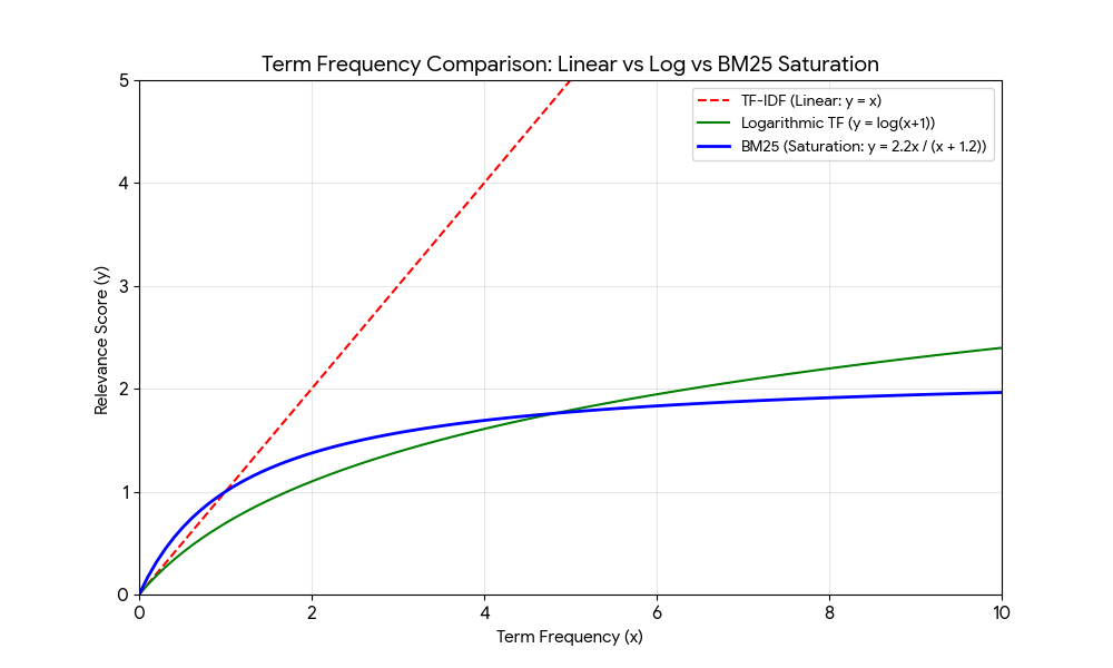 As we can see on the plot above, in TF-IDF word meaning increasing linear, but with BM25 like logarithmic.
This behavior solve the "saturated term frequency" problem. In TF-IDF, if a term appears 100 times, it’s 100x more important. In BM25, after a certain point (controlled by k), more occurrences barely increase the score.
As we can see on the plot above, in TF-IDF word meaning increasing linear, but with BM25 like logarithmic.
This behavior solve the "saturated term frequency" problem. In TF-IDF, if a term appears 100 times, it’s 100x more important. In BM25, after a certain point (controlled by k), more occurrences barely increase the score.
Sentence BERT (Dense Retrieval)
 While BM25 relies on exact word overlaps (Sparse Vectors), SBERT represents sentences in a high-dimensional continuous space (Dense Vectors). In SBERT we calculate the similarity of sentences by measure the angles between the vectors, and thus we find the nearest vector.
The SBERT flow:
While BM25 relies on exact word overlaps (Sparse Vectors), SBERT represents sentences in a high-dimensional continuous space (Dense Vectors). In SBERT we calculate the similarity of sentences by measure the angles between the vectors, and thus we find the nearest vector.
The SBERT flow:
- Embedding: Text passed through a Transformer
- Pooling: Token-level outputs are averaged to create a single "Sentence Embedding."
- Similarity: We measure the cosine similarity between vectors
a = """Abstract
The IRC (Internet Relay Chat) protocol is for use with text based
conferencing."""

b = """Document defines the Client Protocol, and assumes that the
reader is familiar with the IRC Architecture [IRC-ARCH]."""

c = """This document defines the Client Protocol, and assume that
reader familiar with the IRC Architecture """

from sentence_transformers import SentenceTransformer
from sklearn.metrics.pairwise import cosine_similarity
import numpy as np

model = SentenceTransformer('BAAI/bge-small-en-v1.5')
sentence_embeddings = model.encode([a,b,c])

scores = np.zeros((sentence_embeddings.shape[0],sentence_embeddings.shape[0]))
for i in range(sentence_embeddings.shape[0]):
    scores[i,:] = cosine_similarity(
        [sentence_embeddings[i]],
        sentence_embeddings
    )[0]
[[0.99999988 0.67196679 0.72217882]
[0.67196679 1.00000024 0.94958812]
[0.7221787 0.94958794 1.00000012]]As we can see here each sentence close to itself in 100%, and sentence 2 close to 3 about 94%, because they just have different semantic , but they describes same things.
Conclusion
While TF-IDF and BM25 used for lexical(sparse) search based on exact word matches, SBERT is used for semantic(dense) search based on meaning.
SBERT is slower than traditional Keyword Search, because it requires model inference to transform text into vectors, but it provides significantly more relevant results by understanding context.